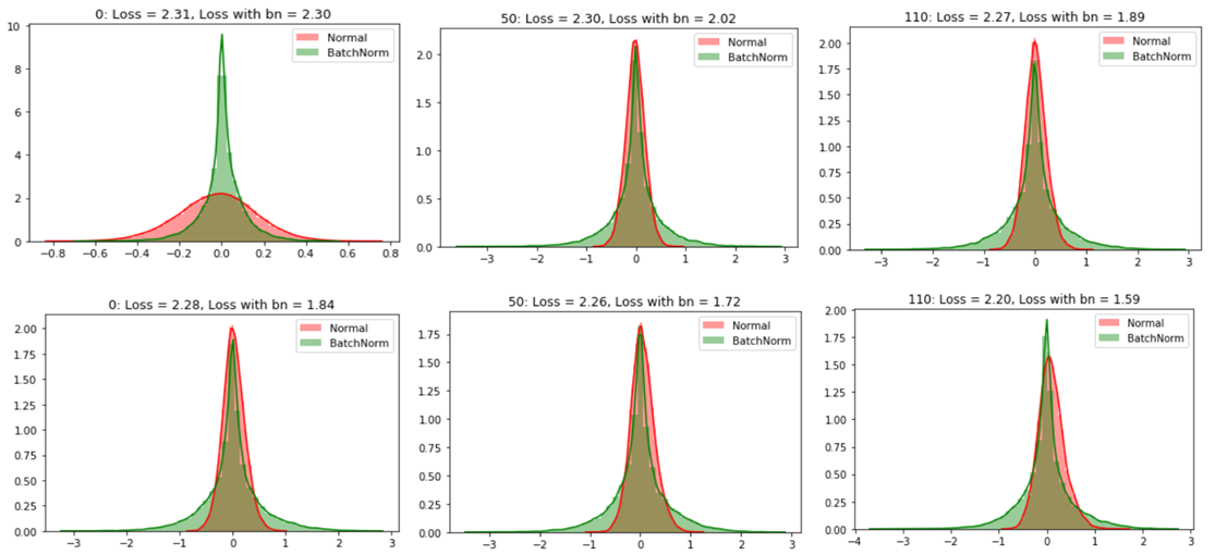
In this article, we will discuss why we need batch normalization and dropout in deep neural networks followed by experiments using Pytorch on a standard data set to see the effects of batch normalization and dropout. This article is based on my understanding of deep learning lectures from PadhAI.
Citation Note: The content and the structure of this article is based on the deep learning lectures from One-Fourth Labs — PadhAI.
Before we discuss batch normalization, we will learn about why normalizing the inputs speed up the training of a neural network.
Consider a scenario where we have 2D data with features x_1 and x_2 going into a neural network. One of these features x_1 has a wider spread from -200 to 200 and another feature x_2 has a narrower spread from -10 to 10.

Once we normalized the data, the spread of the data for both the features is concentrated in one region ie… from -2 to 2. Spread would look like this,

Let’s discuss why normalizing inputs help?
Before we normalized the inputs, the weights associated with these inputs would vary a lot because the input features present in different ranges varying from -200 to 200 and from -2 to 2. To accommodate this range difference between the features some weights would have to be large and then some have to be small. If we have larger weights then the updates associated with the back-propagation would also be large and vice versa. Because of this uneven distribution of weights for the inputs, the learning algorithm keeps oscillating in the plateau region before it finds the global minima.
To avoid the learning algorithm spend much time oscillating in the plateau, we normalize the input features such that all the features would be on the same scale. Since our inputs are on the same scale, the weights associated with them would also be on the same scale. Thus helping the network to train faster.
We have normalized the inputs but what about hidden representatives?
By normalizing the inputs we are able to bring all the inputs features to the same scale. In the neural network, we need to compute the pre-activation for the first neuron of the first layer a₁₁. We know that pre-activation is nothing but the weighted sum of inputs plus bias. In other words, it is the dot product between the first row of the weight matrix W₁ and the input matrix X plus bias b₁₁.

The mathematical equation for pre-activation at each layer ‘i’ is given by,

The activation at each layer is equal to applying the activation function to the output of the pre-activation of that layer. The mathematical equation for the activation at each layer ‘i’ is given by,

Similarly, the activation values for ‘n’ number of hidden layers present in the network need to be computed. The activation values will act as an input to the next hidden layers present in the network. so it doesn’t matter what we have done to the input whether we normalized them or not, the activation values would vary a lot as we do deeper and deeper into the network based on the weight associated with the corresponding neuron.
In order to bring all the activation values to the same scale, we normalize the activation values such that the hidden representation doesn’t vary drastically and also helps us to get improvement in the training speed.
Why is it called batch normalization?
Since we are computing the mean and standard deviation from a single batch as opposed to computing it from the entire data. Batch normalization is done individually at each hidden neuron in the network.

Since we are normalizing all the activations in the network, are we enforcing some constraints that could deteriorate the performance of the network?
In order to maintain the representative power of the hidden neural network, batch normalization introduces two extra parameters — Gamma and Beta. Once we normalize the activation, we need to perform one more step to get the final activation value that can be feed as the input to another layer.

The parameters Gamma and Beta are learned along with other parameters of the network. If Gamma (γ) is equal to the mean (μ) and Beta (β) is equal to the standard deviation(σ) then the activation h_final is equal to the h_norm, thus preserving the representative power of the network.
